Geographical variation in Critical Care bed capacity (Part 1)
- 11 minsI’ve always wondered if there was variation across the UK with regards to Critical Care bed capacity. In other words, are there regions in the UK where there are more Critical Care beds per population than others?
There’re publicly available datasets which we can use to try and answer this question:
- NHS England hosts data on the Critical Care capacity by month and by trust.
- The Office of National Statistics hosts estimates on the population sizes in the different Clinical Commissioning Groups.
- NHS Choices hosts a list of all the Trusts and Hospitals in England with their Latitude and Longitude codes.
- Lastly NHS England hosts a .kml file for all the CCG regions, which we would need to join the data together by region. Unfortunately it’s difficult to read
.kmlfiles into R, and there’re workarounds to do this, but I decided to convert.kmlfile into a.GeoJSONfile using QGIS.
#Load the required packages
library(dplyr)
library(readxl)
library(rgdal)
library(sp)
library(ggplot2)

#Load the data
CC_beds <- read_excel("../data/MSitRep-October-2016-1VHw9.xls", skip = 14)[3:155,2:4] %>%
  rename(beds = `Number of Adult critical care beds`)
#Load the trust data with Latitude and Longitude coordinates
trust <- read.csv("../data/trust.csv")
#Join the two to get the latitude and longitude codes
CC_beds <- left_join(CC_beds, trust, by = c("Code" = "OrganisationCode" )) %>%
select(Code, HospitalName = Name, beds, Latitude, Longitude)
#There are some Trusts with NA values for Latitude and Longitude
#This is likely because the Trusts operate over a number of sites
#To get around this we have to use different Hospital data and get the geometric mean coordinates
hospitals <- read.csv("../data/Hospital 20160921.csv")
x <- CC_beds %>% filter(is.na(Latitude)) %>%
left_join(hospitals, by = c("Code" = "ParentODSCode")) %>%
select(Code, HospitalName, beds, Latitude = Latitude.y, Longitude = Longitude.y) %>%
group_by(Code) %>%
summarise(Latitude = mean(Latitude), Longitude = mean(Longitude))
CC_beds <- CC_beds %>% filter(is.na(Latitude)) %>%
select(-Latitude, -Longitude) %>%
left_join(x, by = "Code") %>%
rbind(CC_beds %>% filter(!is.na(Latitude)))
#Join the coordinates to the CC_beds
CCG_pop <- read_excel("../data/SAPE18DT5-mid-2015-ccg-syoa-estimates.xls", skip = 4, sheet = 2)[c(7:18, 21:31, 34:53, 56:78, 83:96, 99:113, 116:133, 136:149, 154:185, 190:198, 201:214, 217:236, 239:245),c(1, 4:5)]colnames(CCG_pop) <- c("code", "CCG", "pop")
#Load the map
#Make sure you have the right OGR drivers installed by typing "GeoJSON" %in% ogrDrivers()$name
map <- readOGR("../data/CCG_BSC_Apr2015.geojson", "OGRGeoJSON")## OGR data source with driver: GeoJSON
## Source: "../data/CCG_BSC_Apr2015.geojson", layer: "OGRGeoJSON"
## with 209 features
## It has 11 fieldsmap$Name <- gsub("&", "and", map$Name)
map$Name <- gsub("Airedale, Wharfdale and Craven", "Airedale, Wharfedale and Craven", map$Name)
map$Name <- gsub("South East Staffs and Seisdon Peninsular", "South East Staffordshire and Seisdon Peninsula", map$Name)
map$Name <- gsub("North, East, West Devon", "Northern, Eastern and Western Devon", map$Name)
map$Name <- paste("NHS", map$Name)
map$Name <- toupper(map$Name)
map[which(map$Name == "NHS WEST LONDON (KANDC AND QPP)"),1] <- "NHS WEST LONDON"
CCG_pop$CCG <- gsub("&", "and", CCG_pop$CCG)
CCG_pop$CCG <- toupper(CCG_pop$CCG)
#x <- sp::merge(map, CCG_pop, by.x = "Name", by.y = "CCG")So now we have all the data loaded up. We can have a look at what we have visually:
plot(map)
points(x = CC_beds$Longitude, y = CC_beds$Latitude, col = "red", pch = 19)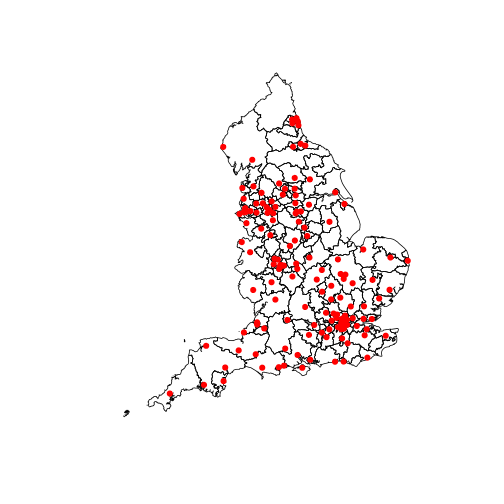
Not very pretty at the moment, but essentially the polygons represent the CCG regions in England, and each red dot represents a Trust with Critical Care beds.
The next step would be to do a spatial join. To find out how many Critical Care beds there are in each CCG region.
CC_beds_sp <- CC_beds
coordinates(CC_beds_sp) <- ~ Longitude + Latitude
proj4string(CC_beds_sp) <- CRS("+proj=longlat +ellps=WGS84 +towgs84=0,0,0,0,0,0,0 +no_defs")
CC_beds <- cbind(CC_beds, over(CC_beds_sp, map))
CCG_CC_beds_join <- CC_beds %>% group_by(Name) %>%
  summarise(sum(beds)) %>%
  left_join(CCG_pop, by = c("Name" = "CCG")) %>%
  rename(crit_care_beds = `sum(beds)`) %>%
  mutate(crit_care_beds_per_pop = crit_care_beds/pop * 100000) # calculate number of beds per 100k pop

nrow(CCG_CC_beds_join)
## [1] 124head(CCG_CC_beds_join)## # A tibble: 6 ? 5
## Name crit_care_beds code pop
## <chr> <dbl> <chr> <dbl>
## 1 NHS AIREDALE, WHARFEDALE AND CRAVEN 7 E38000001 159311
## 2 NHS BARKING AND DAGENHAM 46 E38000004 201979
## 3 NHS BARNSLEY 11 E38000006 239319
## 4 NHS BASILDON AND BRENTWOOD 34 E38000007 257778
## 5 NHS BATH AND NORTH EAST SOMERSET 13 E38000009 184874
## 6 NHS BEDFORDSHIRE 11 E38000010 440274
## # ... with 1 more variables: crit_care_beds_per_pop <dbl>tail(CCG_CC_beds_join)## # A tibble: 6 ? 5
## Name crit_care_beds code pop crit_care_beds_per_pop
## <chr> <dbl> <chr> <dbl> <dbl>
## 1 NHS WEST NORFOLK 13 E38000203 174146 7.465001
## 2 NHS WEST SUFFOLK 9 E38000204 226258 3.977760
## 3 NHS WIGAN BOROUGH 11 E38000205 322022 3.415916
## 4 NHS WILTSHIRE 10 E38000206 486093 2.057220
## 5 NHS WIRRAL 17 E38000208 320900 5.297600
## 6 NHS WOLVERHAMPTON 28 E38000210 254406 11.006030Some CCGs have zero Critical Care Beds.
Let’s now plot a choropleth!
#We will first need to fortify the map SpatialPolygonsDataframe so that ggplot2 can plot it
map.f <- fortify(map, region = "Name")

#Now let's merge the Critical Care Beds data
merge.map.f <- merge(map.f, CCG_CC_beds_join, by.x = "id", by.y = "Name", all.x=TRUE) #%>%
  #mutate(crit_care_beds_per_pop = replace(crit_care_beds_per_pop, which(is.na(crit_care_beds_per_pop)), 0)) %>%
  #mutate(crit_care_beds = replace(crit_care_beds, which(is.na(crit_care_beds)), 0))

#Reorder otherwise the plot will look weird
final.plot <- merge.map.f[order(merge.map.f$order), ]

#Plot!
ggplot() +
  geom_polygon(data = final.plot, aes(x = long, y = lat, group = group, fill = crit_care_beds),
               color = "black", size = 0.1) +
  coord_map() +
  theme_minimal()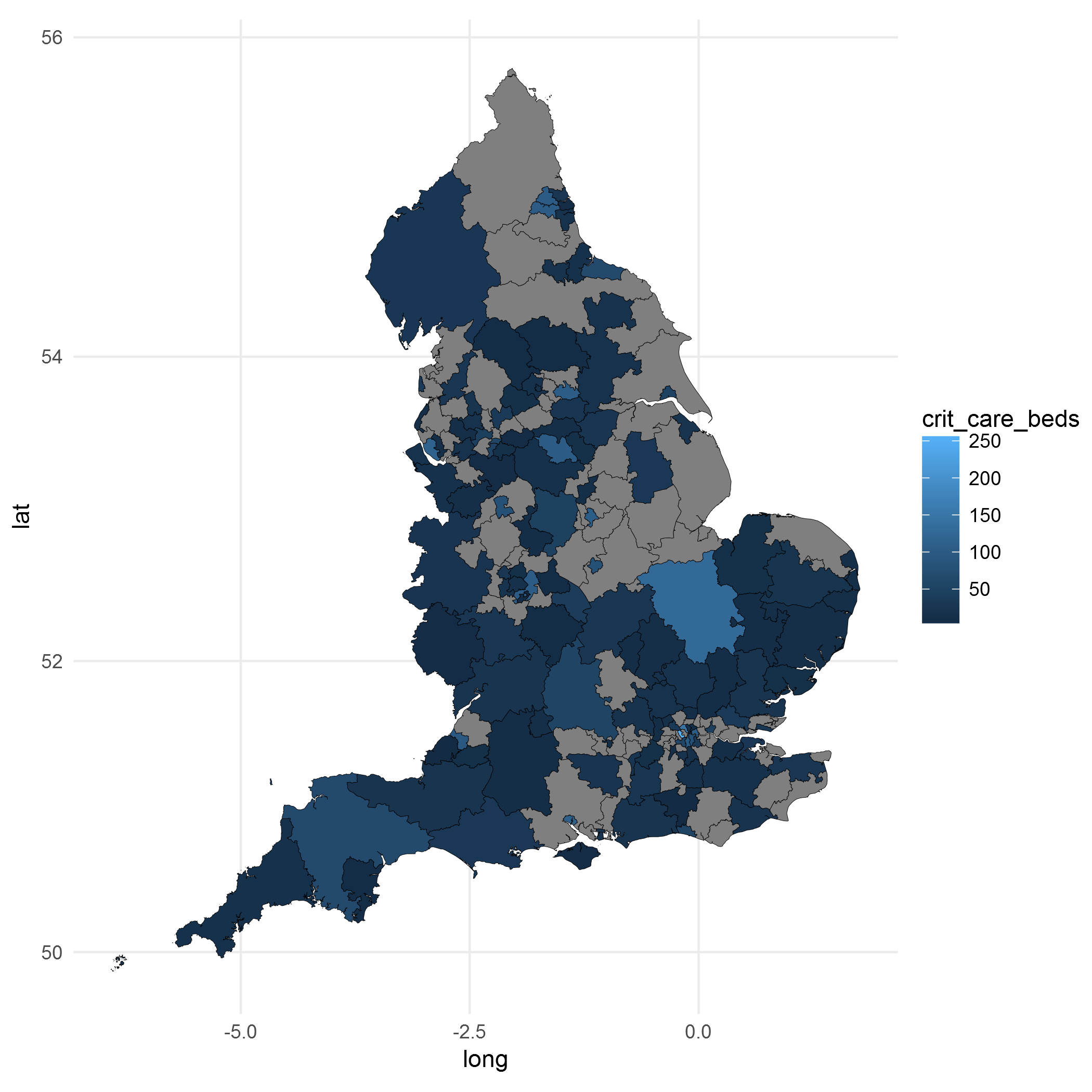
ggplot() +
  geom_polygon(data = final.plot, aes(x = long, y = lat, group = group, fill = crit_care_beds_per_pop),
               color = "black", size = 0.1) +
  coord_map() +
  theme_minimal()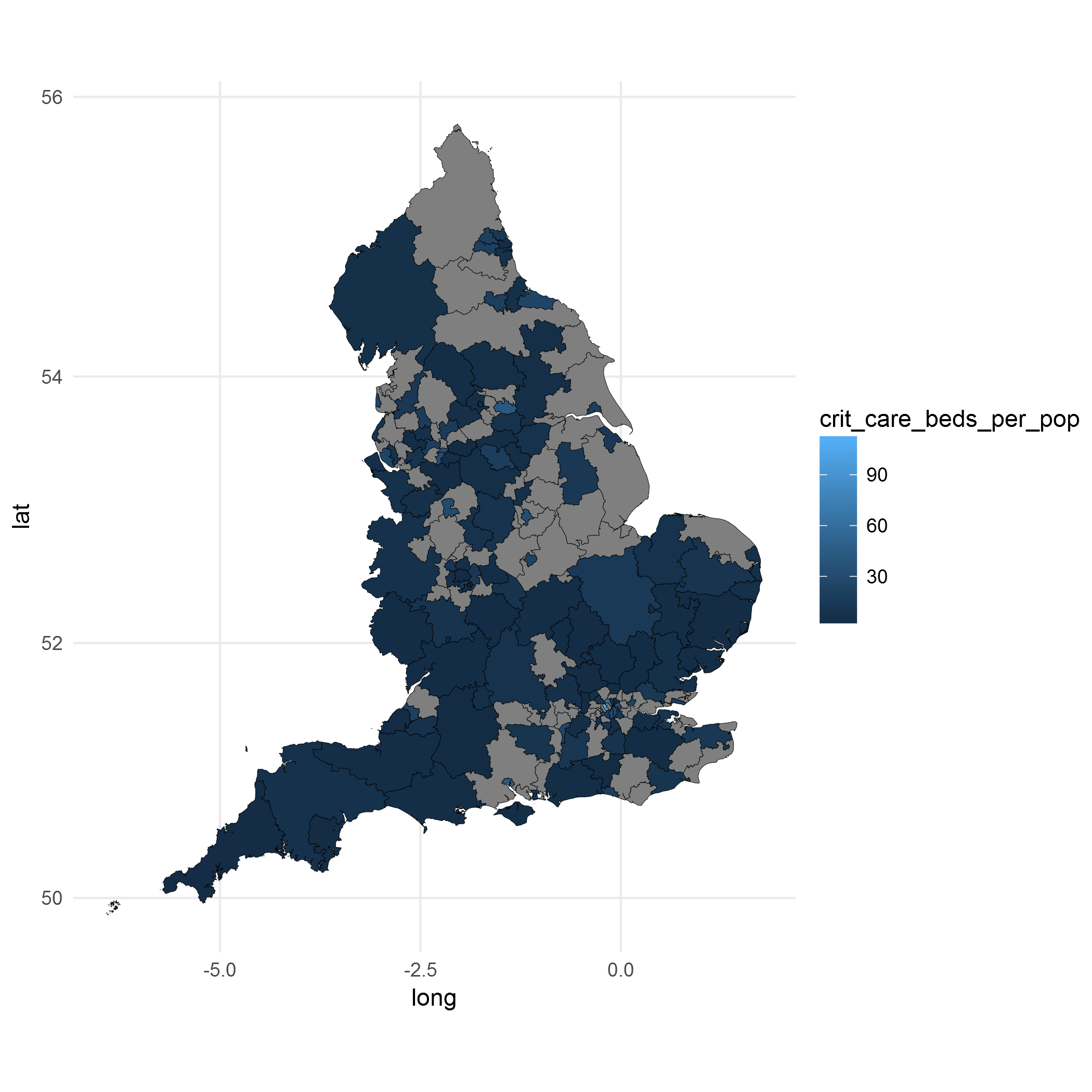
sessionInfo()## R version 3.3.1 (2016-06-21)
## Platform: x86_64-w64-mingw32/x64 (64-bit)
## Running under: Windows >= 8 x64 (build 9200)
##
## locale:
## [1] LC_COLLATE=English_United Kingdom.1252
## [2] LC_CTYPE=English_United Kingdom.1252
## [3] LC_MONETARY=English_United Kingdom.1252
## [4] LC_NUMERIC=C
## [5] LC_TIME=English_United Kingdom.1252
##
## attached base packages:
## [1] stats graphics grDevices utils datasets methods base
##
## other attached packages:
## [1] knitr_1.14 ggplot2_2.1.0.9001 rgdal_1.2-4
## [4] readxl_0.1.1 dplyr_0.5.0 sp_1.2-3
##
## loaded via a namespace (and not attached):
## [1] Rcpp_0.12.7 magrittr_1.5 maptools_0.8-40
## [4] maps_3.1.1 munsell_0.4.3 colorspace_1.2-6
## [7] lattice_0.20-33 R6_2.1.2 stringr_1.0.0
## [10] plyr_1.8.4 tools_3.3.1 grid_3.3.1
## [13] gtable_0.2.0 DBI_0.5 rgeos_0.3-21
## [16] lazyeval_0.2.0 assertthat_0.1 digest_0.6.10
## [19] tibble_1.2 formatR_1.4 mapproj_1.2-4
## [22] evaluate_0.9 labeling_0.3 stringi_1.1.1
## [25] scales_0.4.0.9003 foreign_0.8-66
Danny Wong
Anaesthetist & Health Services Researcher