Linear Regression in R
- 9 minsI recently attended an excellent Introduction to Regression Analysis course run by the Centre for Applied Statistics Courses at UCL. They taught the course with example output from SPSS, so here I try to replicate their steps in R.
The data they provided is simulated and in an Microsoft Excel (.xls) spreadsheet format and can be found here. So let’s start by loading it into R.
#We will use the readxl package to read the data into R
library(readxl)
data <- read_excel("../data/DataSetFile.xls")

#The last 2 rows need to be removed, because they are actually annotations describing the dataset. The first column can be removed because they are just observation numbers.
data <- data[1:42, 2:9]

#We need to tell R that there are some categorical variables
data$female <- as.factor(as.integer(data$female))
data$drugstat <- as.factor(as.integer(data$drugstat))
data$ethnic <- as.factor(as.integer(data$ethnic))
So now we have a dataframe of 42 observations and 8 variables:
-
frcmax= VmaxFRC(L/s), a measure of small airway function of the baby at birth -
female= 0 (male), 1 (female) -
drugstat= Whether the mother was administered pethidine during labour: 0 (No), 1 (Yes) -
heellen= Crown-Heel length (cm) of the baby -
gestag= Gestational age (weeks) at birth -
ethnic= Ethnicity: 0 (White Caucasian), 1 (Black African), 2 (Asian) -
cd4= CD4 count (per mm^3) of the baby -
bwt= Birthweight (grams) of the baby
We will use regression to answer the question: “Is there any association between the use of pethidine during labour and VmaxFRC of the baby at birth?”
We start by examining the variables, getting a general feel of the data.
library(Hmisc) #We will use a function from this package which contains many useful functions for data analysis
library(car) #We will use this package to run a scatterplot matrix
describe(data)
## data
##
## 8 Variables 42 Observations
## ---------------------------------------------------------------------------
## frcmax
## n missing unique Info Mean .05 .10 .25 .50
## 41 1 39 1 100.7 33.2 48.4 69.7 92.9
## .75 .90 .95
## 123.0 152.0 181.0
##
## lowest : 17.5 31.0 33.2 47.9 48.4
## highest: 152.0 175.0 181.0 182.0 220.0
## ---------------------------------------------------------------------------
## female
## n missing unique
## 40 2 2
##
## 0 (20, 50%), 1 (20, 50%)
## ---------------------------------------------------------------------------
## drugstat
## n missing unique
## 41 1 2
##
## 0 (31, 76%), 1 (10, 24%)
## ---------------------------------------------------------------------------
## heellen
## n missing unique Info Mean .05 .10 .25 .50
## 41 1 12 0.98 46.1 43 43 45 46
## .75 .90 .95
## 48 49 51
##
## 40 41 43 44 45 46 47 48 49 50 51 52
## Frequency 1 1 5 3 8 5 7 4 3 1 2 1
## % 2 2 12 7 20 12 17 10 7 2 5 2
## ---------------------------------------------------------------------------
## gestag
## n missing unique Info Mean .05 .10 .25 .50
## 42 0 12 0.99 36.88 32.05 33.10 35.00 37.00
## .75 .90 .95
## 39.00 40.00 41.00
##
## 31 32 33 34 35 36 37 38 39 40 41 42
## Frequency 1 2 2 3 4 6 8 4 3 5 3 1
## % 2 5 5 7 10 14 19 10 7 12 7 2
## ---------------------------------------------------------------------------
## ethnic
## n missing unique
## 42 0 3
##
## 0 (7, 17%), 1 (21, 50%), 2 (14, 33%)
## ---------------------------------------------------------------------------
## cd4
## n missing unique Info Mean .05 .10 .25 .50
## 20 22 20 1 3.389 2.523 2.658 2.783 3.542
## .75 .90 .95
## 4.080 4.435 4.507
##
## lowest : 0.300 2.640 2.660 2.719 2.734
## highest: 4.147 4.364 4.427 4.500 4.634
## ---------------------------------------------------------------------------
## bwt
## n missing unique Info Mean .05 .10 .25 .50
## 42 0 40 1 1994 1385 1433 1778 2042
## .75 .90 .95
## 2260 2457 2526
##
## lowest : 1100 1190 1385 1390 1420, highest: 2460 2501 2527 2580 2590
## ---------------------------------------------------------------------------scatterplotMatrix(~frcmax + heellen + gestag + cd4 + bwt, diagonal = "density", smoother = FALSE, data = data)
stripchart(frcmax ~ drugstat, vertical = TRUE, offset = .5, pch = 19, ylab = "FRC Max", xlab = "Whether Pethidine was given", data = data)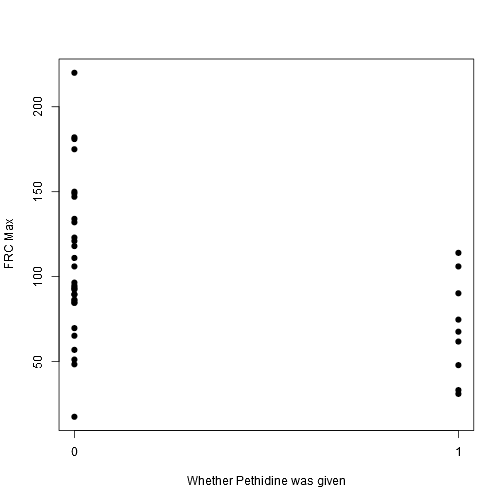
stripchart(frcmax ~ ethnic, vertical = TRUE, offset = .5, pch = 19, ylab = "FRC Max", xlab = "Ethnicity", data = data)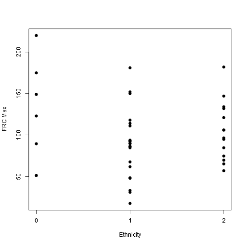
stripchart(frcmax ~ female, vertical = TRUE, offset = .5, pch = 19, ylab = "FRC Max", xlab = "Sex", data = data)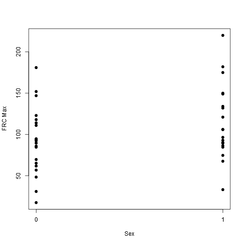
We can now try to fit a linear model, our outcome variable of interest is frcmax, and we need to include the predictor drugstat in our model. But let’s first fit this model frcmax = a + b(bwt)
model1 <- lm(frcmax ~ bwt, data = data)
summary(model1)
##
## Call:
## lm(formula = frcmax ~ bwt, data = data)
##
## Residuals:
## Min 1Q Median 3Q Max
## -76.689 -25.798 -4.778 28.878 103.291
##
## Coefficients:
## Estimate Std. Error t value Pr(>|t|)
## (Intercept) 26.62897 34.78117 0.766 0.4485
## bwt 0.03722 0.01716 2.169 0.0363 *
## ---
## Signif. codes: 0 '***' 0.001 '**' 0.01 '*' 0.05 '.' 0.1 ' ' 1
##
## Residual standard error: 42.58 on 39 degrees of freedom
## (1 observation deleted due to missingness)
## Multiple R-squared: 0.1076, Adjusted R-squared: 0.08474
## F-statistic: 4.703 on 1 and 39 DF, p-value: 0.03626plot(frcmax ~ bwt, pch = 19, data = data)
abline(model1)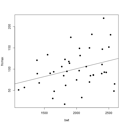
Now let’s add a few more predictors and include the drugstat variable.
model2 <- lm(frcmax ~ bwt + gestag + factor(ethnic) + drugstat, data = data)
summary(model2)
##
## Call:
## lm(formula = frcmax ~ bwt + gestag + factor(ethnic) + drugstat,
## data = data)
##
## Residuals:
## Min 1Q Median 3Q Max
## -72.614 -18.792 -3.731 17.483 80.167
##
## Coefficients:
## Estimate Std. Error t value Pr(>|t|)
## (Intercept) 226.13882 92.83294 2.436 0.0202 *
## bwt 0.07550 0.02323 3.250 0.0026 **
## gestag -6.48755 3.32436 -1.952 0.0593 .
## factor(ethnic)1 -46.91154 19.53192 -2.402 0.0219 *
## factor(ethnic)2 -27.22016 18.62705 -1.461 0.1531
## drugstat1 -17.43254 15.62062 -1.116 0.2722
## ---
## Signif. codes: 0 '***' 0.001 '**' 0.01 '*' 0.05 '.' 0.1 ' ' 1
##
## Residual standard error: 36.42 on 34 degrees of freedom
## (2 observations deleted due to missingness)
## Multiple R-squared: 0.4108, Adjusted R-squared: 0.3241
## F-statistic: 4.741 on 5 and 34 DF, p-value: 0.002158So what does this mean?
In this model, the equation is frcmax = 226.14 + 0.08(bwt) - 6.49(gestag) - 49.91(ethnic = African) - 27.22(ethnic = Asian) - 17.43(drugstat = 1).
The Adjusted R^2 is 0.3241, meaning 32.41% of the variability of frcmax can be accounted for by the predictors in the model. bwt and ethnic = African had p-values <0.05, meaning these were significant independent predictors of frcmax. For every 1 unit increase in bwt, there is a 6.49 unit increase in frcmax, and ethnic = African resulted in a mean frcmax of -46.91 compared to ethnic = White Caucasian.
Since the p-value for drugstat = 1 is 0.2722, it means that after adjusting for the other variables bwt, gestag, ethnic in this model, the null hypothesis is true and there is no statistically significantassociation between the use of pethidine during labour and VmaxFRC of the baby at birth.

Danny Wong
Anaesthetist & Health Services Researcher