Predicting Postoperative Morbidity in Adult Elective Surgical Patients using the Surgical Outcome Risk Tool (SORT)

I recently had a paper published in the British Journal of Anaesthesia, with the same title as this post. Unfortunately it exists behind a paywall as we could not afford the open access charges, but I thought I’d post the source code for the manuscript here. To see the accepted manuscript version of the paper in the UCL Discovery repository, click here.

Like I did for one of my previous papers, I prepared the manuscript in R Markdown. Today I’ll highlight 2 things about the code in the manuscript.

Firstly, here is the code I used to generate the figures used in the paper (Figures 2 and 3) below. Unfortunately I wasn’t able to produce the patient flow diagram (Figure 1) programmatically, and resorted to drawing it up in Microsoft PowerPoint.

#pdf("figures/figure2.pdf", colormodel="cmyk", width = 8, height = 4)
#postscript("figures/figure2.eps", horizontal = FALSE, onefile = FALSE, colormodel="cmyk", paper = "special", height = 4, width = 8)
HL_lrpoms9df <- HL_lrpoms9$Table_HLtest %>% as.data.frame()
HL_possum_morbdf <- HL_possum_morb$Table_HLtest %>% as.data.frame()

par(mar=c(4, 4, 2, 2)+.1,
    mgp=c(2.5, 1, 0))
par(mfrow=c(1,2))
#plot(roc_SORT, col="blue", main="A. SORT vs. P-POSSUM & SRS", 
#     ylim=c(0,1),
#     legacy.axes=TRUE)
#plot(roc_pPOSSUM, col="green", lty = 2, add=TRUE)
#plot(roc_SRS, col="magenta", lty = 4, add=TRUE)
#legend("bottomright", inset = c(0.05,0.05), legend = c("SORT","P-POSSUM","SRS"),
#       col = c("blue","green","magenta"), lty = c(1,2,4),
#       cex = 0.5)

plot(NULL,main="A. Calibration plots",
     asp=1, 
     xlim = c(0,1),
     ylim = c(0,1),
     ylab = "Observed Risk",
     xlab = "Predicted Risk")
abline(a = 0, b = 1, col = "grey", add = TRUE)
points(meanobs ~ meanpred, data = HL_lrpoms9df,
      col = "blue",
      pch = 3, add = TRUE)
#lines(lowess(HL_lrpoms9df$meanpred, HL_lrpoms9df$meanobs, iter = 0), col = "blue", lty = 2)
points(meanobs ~ meanpred, data = HL_possum_morbdf,
      col = "green",
      pch = 2, add = TRUE)
#lines(lowess(HL_possum_morbdf$meanpred, HL_possum_morbdf$meanobs, iter = 0), col = "green", lty = 2)
legend("bottomright", inset = c(0.05,0.05), legend = c("SORT-morbidity","POSSUM"),
       col = c("blue","green"), pch = c(3,2),
       cex = 0.5)
       
plot(roc_model9, col="blue", main="B. ROC curves", 
     ylim=c(0,1),
     legacy.axes=TRUE)
plot(roc_POSSUM, col="green", lty = 2, add=TRUE)
legend("bottomright", inset = c(0.05,0.05), legend = c("SORT-morbidity","POSSUM"),
       col = c("blue","green"), lty = c(1,2),
       cex = 0.5)
par(mfrow=c(1,1))

#dev.off()

That code was used to produce a .pdf file which was then manipulated in GIMP to produce the final .tiff file for submission:

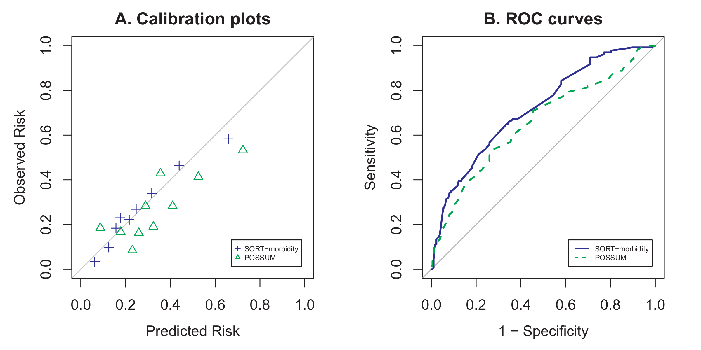
You might wonder why I have commented out one of the graphs (the one labelled “SORT vs. P-POSSUM & SRS”): Essentially that figure existed in one of the earlier versions of the manuscript, but was removed after the first round of peer review, when it became apparent that we did not have enough mortality events in our paper to adequately validate the 3 mortality risk scores in the label.

Secondly, in the first code chunk of my R Markdown document, I have these lines of code:

load("data/SOuRCeDataCleaning.RData")

purl("SOuRCe.Rmd")
read_chunk("SOuRCe.R")
unlink("SOuRCe.R")

What is happening here is, I have written a separate R Markdown document, which I used to clean the original data and save it as an .Rdata file, which I can then load in to this document. I also have a separate SOuRCe.Rmd file which I used to perform all my analysis work, you can look at the code contained within that R Markdown file here, as well as the .html output from that here. This was essentially my analysis for the study, where I conduct all the model development and computing. That document was knitted into either .html or .docx to facilitate analysis discussions with my co-authors during the early days of the study. I then use the purl() function to convert the .Rmd file into .R and I read that code using read_chunk() in my document. Later in the document, I then call parts of the analysis I want to refer to in my manuscript, which are named code chunks. To do so, I include a chunk in my manuscript document like so:

{r, echo=FALSE, message=FALSE, warning=FALSE, results="hide", fig.show='hide'}
<<Ext_val_SORT>>
<<RegressionModel9>>

The <<CodeChunkName>> allows me to just take and run particular named chunks of code from within SOuRCe.Rmd within this second manuscript document. This workflow saved me a huge amount of time! Since I did that work already, I don’t have to rewrite code again when it came to writing the actual manuscript.

Here is an example of this workflow explained by Michael Sachs. He even draws a lovely flow diagram to illustrate the way it works.

sessionInfo()

## R version 3.3.3 (2017-03-06)
## Platform: x86_64-w64-mingw32/x64 (64-bit)
## Running under: Windows >= 8 x64 (build 9200)
## 
## locale:
## [1] LC_COLLATE=English_United Kingdom.1252 
## [2] LC_CTYPE=English_United Kingdom.1252   
## [3] LC_MONETARY=English_United Kingdom.1252
## [4] LC_NUMERIC=C                           
## [5] LC_TIME=English_United Kingdom.1252    
## 
## attached base packages:
## [1] stats     graphics  grDevices utils     datasets  methods   base     
## 
## other attached packages:
## [1] knitr_1.14
## 
## loaded via a namespace (and not attached):
## [1] magrittr_1.5  tools_3.3.3   stringi_1.1.1 stringr_1.2.0 evaluate_0.9

Danny Wong

Anaesthetist & Health Services Researcher

Tweet Share