Looking at Specialty Training Competition Ratios
- 20 minsHealth Education England’s Medical and Dental Recruitment and Selection website publishes the numbers of applicants and available spaces, and hence the competition ratios for each of the Specialties for the last few years of recruitment.
We will try to extract the data and make some inferences. I have borrowed Hadley Wickham’s approach in scraping data from html files.
#Load the required packages
require(rvest) #This package allows us to scrape data from html into R
require(dplyr) #To wrangle data
require(ggplot2) #To plot graphs

#The data for each year is laid out in its own separate page
x2015 <- read_html("http://specialtytraining.hee.nhs.uk/specialty-recruitment/competition-ratios/2015-competition-ratios/") %>%
  html_nodes("table") %>%
  .[[1]] %>%
  html_table()
x2014 <- read_html("http://specialtytraining.hee.nhs.uk/specialty-recruitment/competition-ratios/2014-competition-ratios/") %>%
  html_nodes("table") %>%
  .[[1]] %>%
  html_table() %>%
  select(-X3, -X5) #To remove the 2 columns with empty data
x2013 <- read_html("http://specialtytraining.hee.nhs.uk/specialty-recruitment/competition-ratios/2013-competition-ratios/") %>%
  html_nodes("table") %>%
  .[[1]] %>%
  html_table() %>%
  select(-X3, -X6, -X7)
There are some inconsistencies in the reporting of some of the Specialties between the different years. For example Medical Microbiology is not reported in 2015, but is reported in 2013 and 2014. Similarly Community Sexual and Reproductive Health is reported in 2014 and 2015, but not in 2013. It may be because there wasn’t any recruitment for some Specialties in some years. Also there is some inconsistency in the nomenclature, eg. Anaesthetics is sometimes reported as Anaesthetics (including ACCS Anaesthetics). Let’s join the data into a big table and clean it a little bit.
x2015[2,1] <- "ACCS EM"
x2014[2,1] <- "ACCS EM"
x2013[2,1] <- "ACCS EM"

x2015[3,1] <- "Anaesthetics"
x2014[3,1] <- "Anaesthetics"
x2013[3,1] <- "Anaesthetics"

x2015[4,1] <- "Broad-Based Training"
x2014[4,1] <- "Broad-Based Training"
x2013[4,1] <- "Broad-Based Training"

x2015[8,1] <- "Core Medical Training"
x2014[8,1] <- "Core Medical Training"
x2013[7,1] <- "Core Medical Training"

x2013[8,1] <- "Core Psychiatry Training"

x2014[18,1] <- "Paediatrics"
x2013[16,1] <- "Paediatrics"

#Join up the data into one dataframe
x <- inner_join(x2013, x2014, by = "X1") %>% inner_join(x2015, by = "X1")

#Rename the columns correctly
colnames(x)[1] <- "Specialty"
colnames(x)[2] <- "Apps2013"
colnames(x)[3] <- "Posts2013"
colnames(x)[4] <- "Ratio2013"
colnames(x)[5] <- "Apps2014"
colnames(x)[6] <- "Posts2014"
colnames(x)[7] <- "Ratio2014"
colnames(x)[8] <- "Apps2015"
colnames(x)[9] <- "Posts2015"
colnames(x)[10] <- "Ratio2015"
#Remove the 1st row
x <- x[-1, ]
row.names(x) <- 1:nrow(x)
Let’s see what we are left with.
require(knitr)
kable(x)| Specialty | Apps2013 | Posts2013 | Ratio2013 | Apps2014 | Posts2014 | Ratio2014 | Apps2015 | Posts2015 | Ratio2015 |
|---|---|---|---|---|---|---|---|---|---|
| ACCS EM | 534 | 203 | 2.6 | 759 | 363 | 2.1 | 881 | 363 | 2.43 |
| Anaesthetics | 1189 | 478 | 2.5 | 1262 | 595 | 2.1 | 1294 | 629 | 2.06 |
| Broad-Based Training | 429 | 52 | 8.3 | 258 | 42 | 6.1 | 363 | 83 | 4.37 |
| Clinical Radiology | 751 | 185 | 4.1 | 798 | 227 | 3.5 | 917 | 247 | 3.71 |
| Core Medical Training | 3088 | 1209 | 2.6 | 3065 | 1468 | 2.1 | 2632 | 1550 | 1.7 |
| Core Psychiatry Training | 650 | 437 | 1.5 | 643 | 497 | 1.3 | 662 | 466 | 1.42 |
| Core Surgical Training | 1296 | 676 | 1.9 | 1370 | 625 | 2.2 | 1396 | 604 | 2.31 |
| General Practice | 6447 | 2787 | 2.3 | 5477 | 3391 | 1.6 | 5112 | 3612 | 1.42 |
| Histopathology | 154 | 120 | 1.3 | 165 | 93 | 1.8 | 189 | 79 | 2.39 |
| Neurosurgery | 183 | 37 | 4.9 | 159 | 24 | 6.6 | 169 | 30 | 5.63 |
| Obstetrics and Gynaecology | 591 | 204 | 2.9 | 583 | 240 | 2.4 | 599 | 238 | 2.52 |
| Ophthalmology | 323 | 71 | 4.5 | 353 | 82 | 4.3 | 374 | 95 | 3.94 |
| Paediatrics | 793 | 360 | 2.2 | 814 | 435 | 1.9 | 801 | 446 | 1.8 |
| Public Health | 602 | 70 | 8.6 | 686 | 78 | 8.8 | 724 | 88 | 8.23 |
This is still a little messy. The data is humanly readable, but we can’t really use it for analysis in R. We need to try and tidy things up, and express all the rows as observations (the different years and the different specialties), and columns as the variables in question (number of applications, number of available posts, competition ratios). So let’s do this.
#First let's add a column for the year
x2015 <- mutate(x2015, Year = 2015)
x2014 <- mutate(x2014, Year = 2014)
x2013 <- mutate(x2013, Year = 2013)

#Rename the columns (Could definitely be improved into an apply function)
colnames(x2015)[1] <- "Specialty"
colnames(x2015)[2] <- "Applicants"
colnames(x2015)[3] <- "Posts"
colnames(x2015)[4] <- "Ratio"

colnames(x2014)[1] <- "Specialty"
colnames(x2014)[2] <- "Applicants"
colnames(x2014)[3] <- "Posts"
colnames(x2014)[4] <- "Ratio"

colnames(x2013)[1] <- "Specialty"
colnames(x2013)[2] <- "Applicants"
colnames(x2013)[3] <- "Posts"
colnames(x2013)[4] <- "Ratio"

#Let's drop the first and last rows
x2015 <- x2015[-1, ]
x2015 <- x2015[-18, ]
row.names(x2015) <- 1:nrow(x2015)

#Repeat for the 2014 and 2013 dataframes
x2014 <- x2014[-1, ]
x2014 <- x2014[-19, ]
row.names(x2014) <- 1:nrow(x2014)

x2013 <- x2013[-1, ]
x2013 <- x2013[-17, ]
row.names(x2013) <- 1:nrow(x2013)

#Now we can bind the rows together
CompetitionRatios <- bind_rows(x2013, x2014) %>% bind_rows(x2015)
Now let’s look at the resulting dataframe
require(knitr)
kable(CompetitionRatios)| Specialty | Applicants | Posts | Ratio | Year |
|---|---|---|---|---|
| ACCS EM | 534 | 203 | 2.6 | 2013 |
| Anaesthetics | 1189 | 478 | 2.5 | 2013 |
| Broad-Based Training | 429 | 52 | 8.3 | 2013 |
| Cardiothoracic Surgery (Pilot) | 68 | 6 | 11.3 | 2013 |
| Clinical Radiology | 751 | 185 | 4.1 | 2013 |
| Core Medical Training | 3088 | 1209 | 2.6 | 2013 |
| Core Psychiatry Training | 650 | 437 | 1.5 | 2013 |
| Core Surgical Training | 1296 | 676 | 1.9 | 2013 |
| General Practice | 6447 | 2787 | 2.3 | 2013 |
| Histopathology | 154 | 120 | 1.3 | 2013 |
| Medical Microbiology & Virology | 108 | 21 | 5.1 | 2013 |
| Neurosurgery | 183 | 37 | 4.9 | 2013 |
| Obstetrics and Gynaecology | 591 | 204 | 2.9 | 2013 |
| Ophthalmology | 323 | 71 | 4.5 | 2013 |
| Paediatrics | 793 | 360 | 2.2 | 2013 |
| Public Health | 602 | 70 | 8.6 | 2013 |
| ACCS EM | 759 | 363 | 2.1 | 2014 |
| Anaesthetics | 1262 | 595 | 2.1 | 2014 |
| Broad-Based Training | 258 | 42 | 6.1 | 2014 |
| Cardiothoracic Surgery (Pilot) | 72 | 7 | 10.3 | 2014 |
| Clinical Radiology | 798 | 227 | 3.5 | 2014 |
| Community Sexual and Reproductive Health | 33 | 7 | 4.7 | 2014 |
| Core Medical Training | 3065 | 1468 | 2.1 | 2014 |
| Core Psychiatry Training | 643 | 497 | 1.3 | 2014 |
| Core Surgical Training | 1370 | 625 | 2.2 | 2014 |
| General Practice | 5477 | 3391 | 1.6 | 2014 |
| Histopathology | 165 | 93 | 1.8 | 2014 |
| Medical Microbiology | 50 | 14 | 3.6 | 2014 |
| Neurosurgery | 159 | 24 | 6.6 | 2014 |
| Obstetrics and Gynaecology | 583 | 240 | 2.4 | 2014 |
| Ophthalmology | 353 | 82 | 4.3 | 2014 |
| Oral and Maxillo Facial Surgery (Pilot) | 33 | 4 | 8.25 | 2014 |
| Paediatrics | 814 | 435 | 1.9 | 2014 |
| Public Health | 686 | 78 | 8.8 | 2014 |
| ACCS EM | 881 | 363 | 2.43 | 2015 |
| Anaesthetics | 1294 | 629 | 2.06 | 2015 |
| Broad-Based Training | 363 | 83 | 4.37 | 2015 |
| Cardiothoracic Surgery | 68 | 8 | 8.5 | 2015 |
| Clinical Radiology | 917 | 247 | 3.71 | 2015 |
| Community Sexual and Reproductive Health | 100 | 2 | 50 | 2015 |
| Core Medical Training | 2632 | 1550 | 1.7 | 2015 |
| Core Psychiatry Training | 662 | 466 | 1.42 | 2015 |
| Core Surgical Training | 1396 | 604 | 2.31 | 2015 |
| General Practice | 5112 | 3612 | 1.42 | 2015 |
| Histopathology | 189 | 79 | 2.39 | 2015 |
| Neurosurgery | 169 | 30 | 5.63 | 2015 |
| Obstetrics and Gynaecology | 599 | 238 | 2.52 | 2015 |
| Ophthalmology | 374 | 95 | 3.94 | 2015 |
| Oral and Maxillo Facial Surgery | 27 | 5 | 5.4 | 2015 |
| Paediatrics | 801 | 446 | 1.8 | 2015 |
| Public Health | 724 | 88 | 8.23 | 2015 |
Now we can start doing something with the data.
Let’s now plot some graphs to visualise the data
#Need to first convert the Specialty column from a vector of characters to factors
CompetitionRatios$Specialty <- as.factor(CompetitionRatios$Specialty)
CompetitionRatios$Ratio <- as.numeric(CompetitionRatios$Ratio)
CompetitionRatios$Year <- as.factor(CompetitionRatios$Year)
CompetitionRatios$Applicants <- as.numeric(CompetitionRatios$Applicants)
CompetitionRatios$Posts <- as.numeric(CompetitionRatios$Posts)

ggplot(data=CompetitionRatios, aes(x=Year, y=Ratio, group = Specialty, colour = Specialty)) +
  geom_line()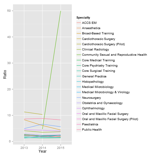
So this is a little busy, it might be worth reducing the number of Specialties to just GP, CMT, CST, Paediatrics and Anaesthetics, the top 5 Specialties by number of applicants in all three years.
#Need to first convert the Specialty column from a vector of characters to factors
CompetitionRatios2 <- CompetitionRatios %>% filter(Specialty == "Anaesthetics" | Specialty == "Core Medical Training" | Specialty == "Core Surgical Training" | Specialty == "General Practice" | Specialty == "Paediatrics")

ggplot(data=CompetitionRatios2, aes(x=Year, y=Ratio, group = Specialty, colour = Specialty)) +
  geom_line() +
  geom_point(aes(shape = factor(Specialty)))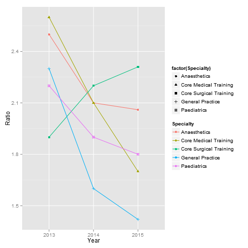
We can immediately see that generally speaking for this group of specialties, other than Core Surgical Training, the Competition Ratio is reducing over these 3 years. Why is this so? Is it due more to dropping applicant numbers or an increase in posts?
Let’s plot the graphs of Applicants over time and Posts over time.
#Need to first convert the Specialty column from a vector of characters to factors
CompetitionRatios2 <- CompetitionRatios %>% filter(Specialty == "Anaesthetics" | Specialty == "Core Medical Training" | Specialty == "Core Surgical Training" | Specialty == "General Practice" | Specialty == "Paediatrics")

ggplot(data=CompetitionRatios2, aes(x=Year, y=Applicants, group = Specialty, colour = Specialty)) +
  geom_line() +
  geom_point(aes(shape = factor(Specialty)))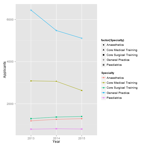
ggplot(data=CompetitionRatios2, aes(x=Year, y=Posts, group = Specialty, colour = Specialty)) +
  geom_line() +
  geom_point(aes(shape = factor(Specialty)))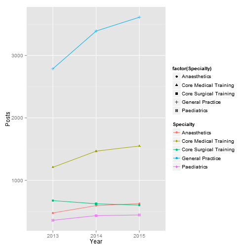
We can see that for GP, and CMT the number of applicants have been dropping year-on-year. Whereas for CST and Anaesthetics, the applicant numbers have been rising slightly. Paediatrics has been relatively static.
However, despite the dropping number of applicants for GP and CMT, there have also been a significant increase year-on-year in the number of available posts for these specialties. Anaesthetics and Paediatrics have also had some increase in their number of posts.
In conclusion, GP and CMT in particular have much less uptake in applicants, seemingly indicating that they are becoming less popular, despite the presumably increasing workforce demands for these two specialties.

Danny Wong
Anaesthetist & Health Services Researcher