Fast food outlets in CCG areas
- 11 minsI’ve always wondered if there was a relationship between the density of fast food outlets in an area and the health outcomes in that area. There are many studies linking the number of fast food outlets in neighbourhoods to obesity rates, Type 2 Diabetes, and cardiovascular outcomes. But these seem to have been done in small areas and not utilising large open data sources.
Openstreetmap (OSM) is a free, open, community-driven mapping initiative which powers many other applications. It has data which is available to download, and updated daily. Geofabrik.de maintains daily mirrors of OSM data that can be downloaded. These include details of all sorts of points of interest, like roads, parks, buildings, etc. Importantly for our purposes, it contains the latitude and longitude codes for fast food outlets! We download the shapefiles for England from here, and I filter out the layer for points of interest, select the fast food outlet coordinates then convert them to a GeoJSON file on QGIS before manipulating them in R.
The reason I convert to GeoJSON is that I previously did this for the CCG maps, when I looked at Critical Care beds, and since I’m going to use them again here, converting to GeoJSON in QGIS saves me the hassle of having to line-up the projections of the spatial dataframes.
Now let’s load up the spatial data.
#Load the required packages
library(dplyr)
library(readxl)
library(rgdal)
library(sp)
library(ggplot2)

#Load the fast food outlet coordinates
fast_food <- readOGR("../data/fast_food.geojson", "OGRGeoJSON")
## OGR data source with driver: GeoJSON
## Source: "../data/fast_food.geojson", layer: "OGRGeoJSON"
## with 12311 features
## It has 4 fields#Load the CCG polygons as we did before
map <- readOGR("../data/CCG_BSC_Apr2015.geojson", "OGRGeoJSON")## OGR data source with driver: GeoJSON
## Source: "../data/CCG_BSC_Apr2015.geojson", layer: "OGRGeoJSON"
## with 209 features
## It has 12 fieldsmap$Name <- gsub("&", "and", map$Name)
map$Name <- gsub("Airedale, Wharfdale and Craven", "Airedale, Wharfedale and Craven", map$Name)
map$Name <- gsub("South East Staffs and Seisdon Peninsular", "South East Staffordshire and Seisdon Peninsula", map$Name)
map$Name <- gsub("North, East, West Devon", "Northern, Eastern and Western Devon", map$Name)
map$Name <- paste("NHS", map$Name)
map$Name <- toupper(map$Name)
map[which(map$Name == "NHS WEST LONDON (KANDC AND QPP)"),1] <- "NHS WEST LONDON"
map$area_sqkm <- raster::area(map) / 1000000
#Check we have it all loaded up correctly
plot(map)
plot(fast_food, add = TRUE, col = "red")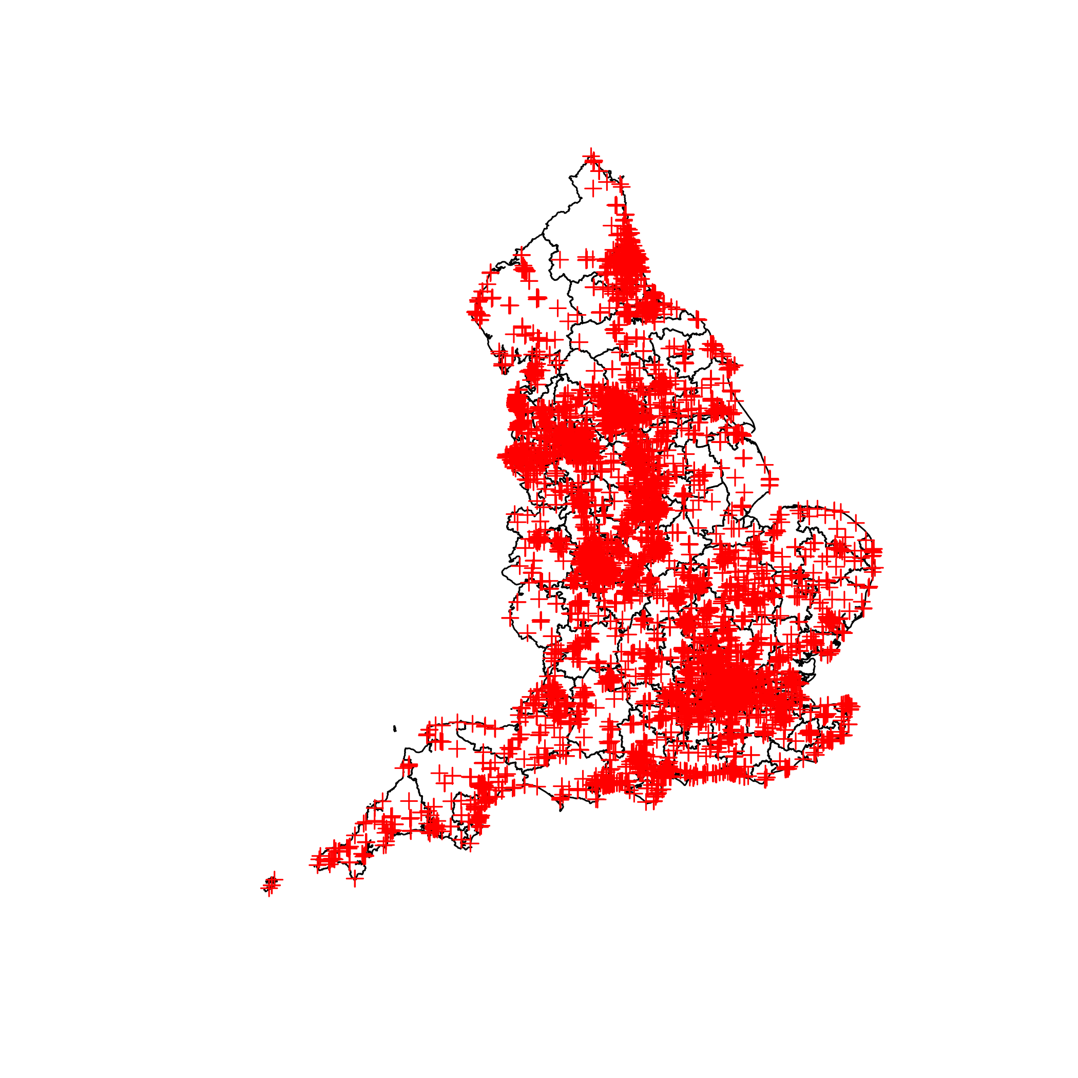
Now that we have the spatial data loaded up we can join them to see how many fast food outlets are in each CCG.
#Perform the join using the sp function over()
fast_food_join <- cbind(as.data.frame(fast_food), over(fast_food, map))

fast_food_table <- table(fast_food_join$Name) %>% as.data.frame() %>% arrange(desc(Freq))
head(fast_food_table)
## Var1 Freq
## 1 NHS BIRMINGHAM CROSSCITY 348
## 2 NHS NOTTINGHAM CITY 309
## 3 NHS NEWCASTLE GATESHEAD 264
## 4 NHS CAMBRIDGESHIRE AND PETERBOROUGH 249
## 5 NHS SANDWELL AND WEST BIRMINGHAM 228
## 6 NHS CUMBRIA 214#Add population data
CCG_pop <- read_excel("../data/SAPE18DT5-mid-2015-ccg-syoa-estimates.xls", skip = 4, sheet = 2)[c(7:18, 21:31, 34:53, 56:78, 83:96, 99:113, 116:133, 136:149, 154:185, 190:198, 201:214, 217:236, 239:245),c(1, 4:5)]## DEFINEDNAME: 21 00 00 01 0b 00 00 00 02 00 00 00 00 00 00 0d 3b 00 00 00 00 fa 00 02 00 02 00
## DEFINEDNAME: 21 00 00 01 0b 00 00 00 02 00 00 00 00 00 00 0d 3b 00 00 00 00 fa 00 02 00 02 00
## DEFINEDNAME: 21 00 00 01 0b 00 00 00 02 00 00 00 00 00 00 0d 3b 00 00 00 00 fa 00 02 00 02 00
## DEFINEDNAME: 21 00 00 01 0b 00 00 00 02 00 00 00 00 00 00 0d 3b 00 00 00 00 fa 00 02 00 02 00colnames(CCG_pop) <- c("code", "CCG", "pop")
CCG_pop$CCG <- gsub("&", "and", CCG_pop$CCG)
CCG_pop$CCG <- toupper(CCG_pop$CCG)
#Join and then calculate the number of fast food outlets per population
fast_food_table <- left_join(fast_food_table, CCG_pop, by = c("Var1" = "CCG")) %>%
mutate(FF_per_pop = Freq/pop*100000) %>%
left_join(as.data.frame(map)[,c("Name", "area_sqkm")], by = c("Var1" = "Name")) %>%
mutate(FF_per_sqkm = Freq/area_sqkm)
head(fast_food_table)## Var1 Freq code pop FF_per_pop
## 1 NHS BIRMINGHAM CROSSCITY 348 E38000012 740797 46.97643
## 2 NHS NOTTINGHAM CITY 309 E38000132 318901 96.89527
## 3 NHS NEWCASTLE GATESHEAD 264 E38000212 493879 53.45439
## 4 NHS CAMBRIDGESHIRE AND PETERBOROUGH 249 E38000026 876367 28.41275
## 5 NHS SANDWELL AND WEST BIRMINGHAM 228 E38000144 487688 46.75120
## 6 NHS CUMBRIA 214 E38000041 504052 42.45594
## area_sqkm FF_per_sqkm
## 1 196.88165 1.76755935
## 2 74.56133 4.14423944
## 3 255.57598 1.03296091
## 4 3760.02641 0.06622294
## 5 118.71390 1.92058378
## 6 6962.48915 0.03073613Now we have a dataframe of fast food outlets per population in each CCG. We can link them to health outcomes.
NHS England tracks a collection of CCG outcomes in the CCG Outcomes Indicator Set (CCGOIS). We can look at the following indicators to start off with:
##Under 75 mortality from cardiovascular disease
fast_food_table <- read.csv("https://indicators.hscic.gov.uk/download/Clinical%20Commissioning%20Group%20Indicators/Data/CCG_1.2_I00754_D.csv") %>%
  filter(Breakdown == "CCG") %>%
  filter(Reporting.period == 2015) %>%
  filter(Gender == "Person") %>%
  select(Level.description, ONS.code, DSR) %>%
  rename(CVS_mort = DSR , CCG = Level.description) %>%
  right_join(fast_food_table, by = c("ONS.code" = "code"))

plot(CVS_mort ~ FF_per_pop, data = fast_food_table)
abline(lm(CVS_mort ~ FF_per_pop, data = fast_food_table))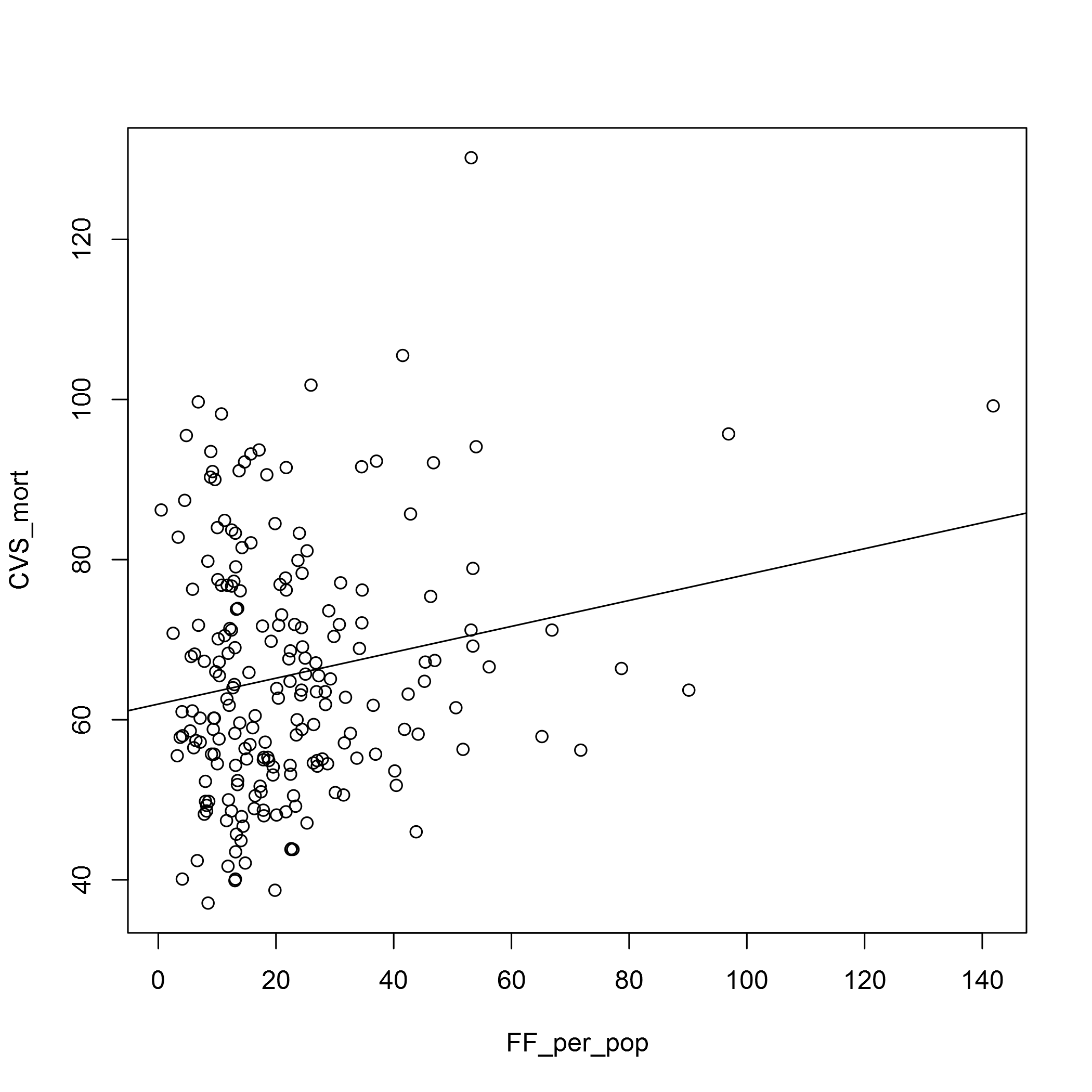
##Under 75 mortality from cancer
fast_food_table <- read.csv("https://indicators.hscic.gov.uk/download/Clinical%20Commissioning%20Group%20Indicators/Data/CCG_1.9_I00756_D.csv") %>%
  filter(Breakdown == "CCG") %>%
  filter(Reporting.period == 2015) %>%
  filter(Gender == "Person") %>%
  select(ONS.code, DSR) %>%
  rename(Cancer_mort = DSR) %>%
  right_join(fast_food_table, by = "ONS.code")

plot(Cancer_mort ~ FF_per_pop, data = fast_food_table)
abline(lm(Cancer_mort ~ FF_per_pop, data = fast_food_table))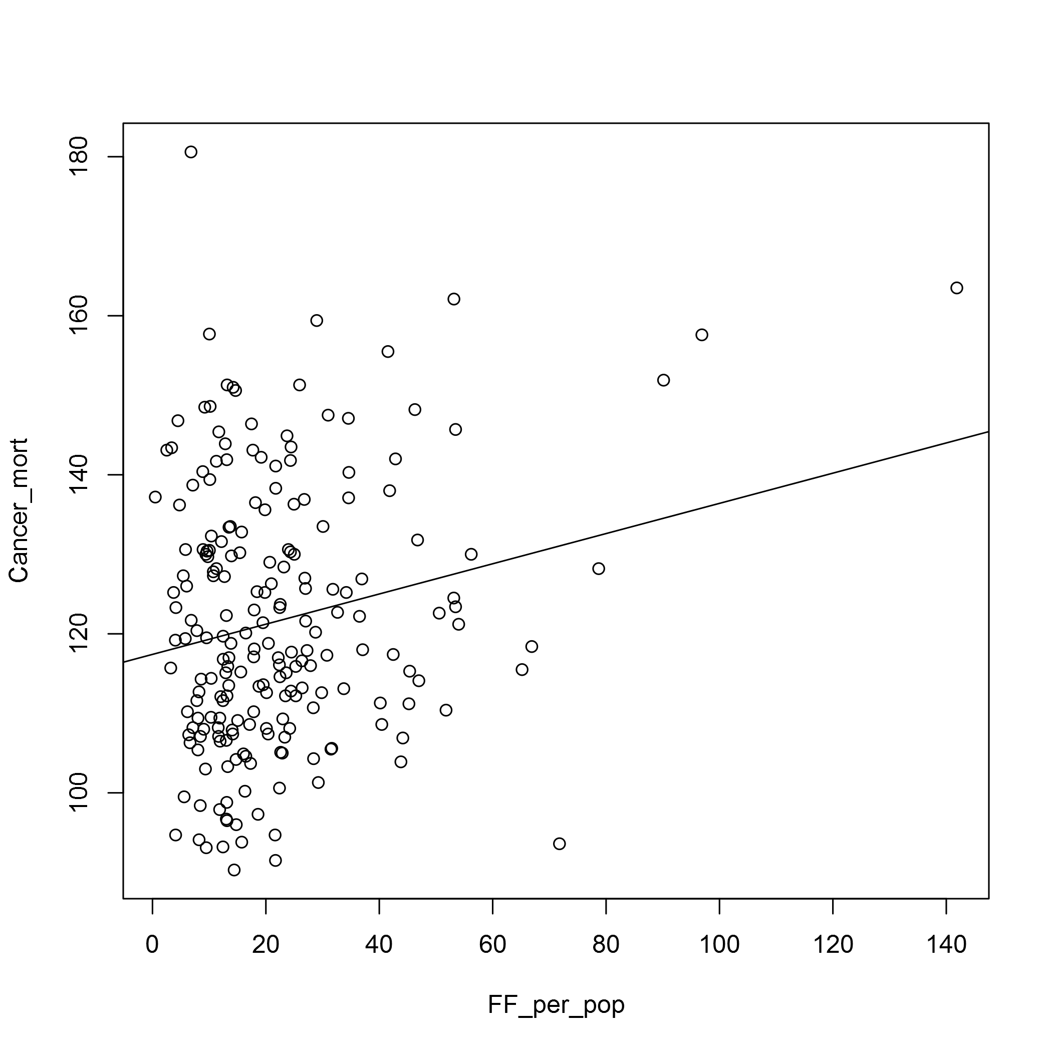
In both cases the relationship doesn’t look very strong. We may have to look at the types of fast food outlets there are, and also the OSM data does seem to have some deficits. In the Barking and Dagenham CCG area, for example, there seems to be too few fast food outlets for it to be believable. I’m sure there is an error in the data there!
fast_food_table %>% select(CCG, Freq) %>% tail()## CCG Freq
## 204 NHS St Helens CCG 6
## 205 NHS Vale Royal CCG 6
## 206 NHS South Sefton CCG 4
## 207 NHS South West Lincolnshire CCG 4
## 208 NHS Corby CCG 3
## 209 NHS Barking and Dagenham CCG 1sessionInfo()## R version 3.3.1 (2016-06-21)
## Platform: x86_64-w64-mingw32/x64 (64-bit)
## Running under: Windows >= 8 x64 (build 9200)
##
## locale:
## [1] LC_COLLATE=English_United Kingdom.1252
## [2] LC_CTYPE=English_United Kingdom.1252
## [3] LC_MONETARY=English_United Kingdom.1252
## [4] LC_NUMERIC=C
## [5] LC_TIME=English_United Kingdom.1252
##
## attached base packages:
## [1] stats graphics grDevices utils datasets methods base
##
## other attached packages:
## [1] ggplot2_2.1.0.9001 rgdal_1.2-4 sp_1.2-3
## [4] readxl_0.1.1 dplyr_0.5.0 knitr_1.14
##
## loaded via a namespace (and not attached):
## [1] Rcpp_0.12.7 raster_2.5-8 magrittr_1.5
## [4] munsell_0.4.3 colorspace_1.2-6 lattice_0.20-33
## [7] R6_2.1.2 plyr_1.8.4 stringr_1.0.0
## [10] tools_3.3.1 grid_3.3.1 gtable_0.2.0
## [13] DBI_0.5 htmltools_0.3.5 lazyeval_0.2.0
## [16] yaml_2.1.13 rprojroot_1.2 digest_0.6.10
## [19] assertthat_0.1 tibble_1.2 formatR_1.4
## [22] evaluate_0.9 rmarkdown_1.3 stringi_1.1.1
## [25] scales_0.4.0.9003 backports_1.0.5
Danny Wong
Anaesthetist & Health Services Researcher