Geographical variation in Critical Care bed capacity (Part 2)

Thursday. December 22, 2016 - 3 mins

In my last post, I started cleaning some openly accessible data to look at whether we can see if there was geographical variation in Critical Care beds.

We ended up with a couple of choropleths which didn’t look that great.

I realise because of the continuous scale, it is quite hard to distinguish between the areas with high density of Critical Care beds vs. those with lower densities. Therefore I have decided to bin the Critical Care beds per 100,000 population into some arbitrarily selected ranges

#Load the required packages
library(dplyr)
library(readxl)
library(rgdal)
library(sp)
library(ggplot2)

Assuming we have already loaded the data we needed from the previous post, we just need to make some categorical variables from the continuous variable of number of Critical Care beds per 100,000 population using the cut() function.

CCG_CC_beds_join <- CCG_CC_beds_join %>% mutate(beds_binned = cut(crit_care_beds_per_pop, c(0,3,5,10,20, Inf)))

table(CCG_CC_beds_join$beds_binned)

## 
##    (0,3]    (3,5]   (5,10]  (10,20] (20,Inf] 
##        8       33       38       26       19

This yields a 5 category scale, which should be easier for the human eye to distinguish.

Finally we replot the map.

map.f <- fortify(map, region = "Name")

#We merge our map with the dataframe again, now containing the binned data
merge.map.f <- merge(map.f, CCG_CC_beds_join, by.x = "id", by.y = "Name", all.x=TRUE) #%>% 

#Reorder otherwise the plot will look weird
final.plot <- merge.map.f[order(merge.map.f$order), ] 

#Plot!
ggplot() +
  geom_polygon(data = final.plot, aes(x = long, y = lat, group = group, fill = beds_binned),
               color = "black", size = 0.1) +
  coord_map() +
  scale_fill_brewer(palette = "Blues") +
  theme_minimal()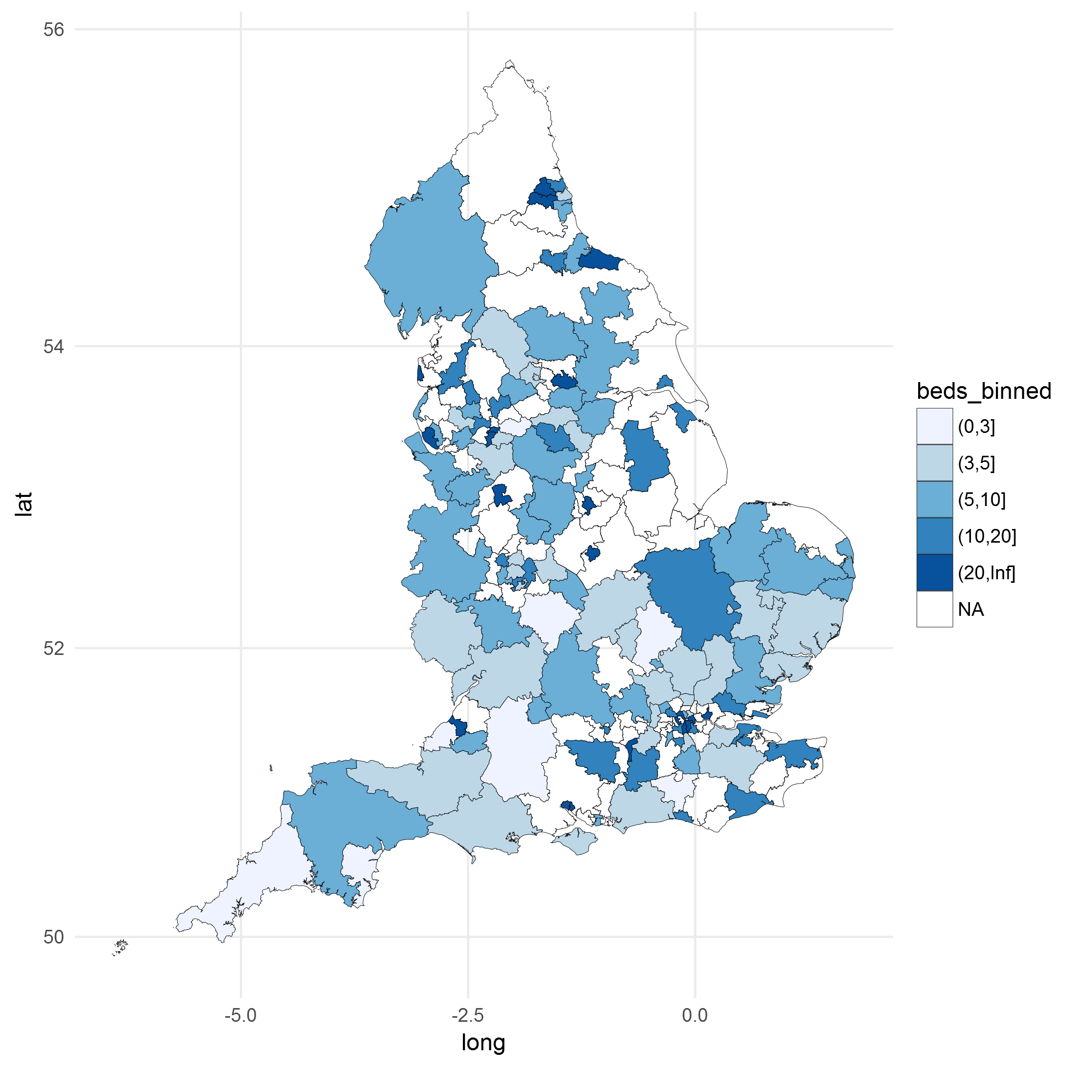

center

I think this map is much better than the previous ones we had.

sessionInfo()

## R version 3.3.1 (2016-06-21)
## Platform: x86_64-w64-mingw32/x64 (64-bit)
## Running under: Windows >= 8 x64 (build 9200)
## 
## locale:
## [1] LC_COLLATE=English_United Kingdom.1252 
## [2] LC_CTYPE=English_United Kingdom.1252   
## [3] LC_MONETARY=English_United Kingdom.1252
## [4] LC_NUMERIC=C                           
## [5] LC_TIME=English_United Kingdom.1252    
## 
## attached base packages:
## [1] stats     graphics  grDevices utils     datasets  methods   base     
## 
## other attached packages:
## [1] ggplot2_2.1.0.9001 rgdal_1.2-4        sp_1.2-3          
## [4] readxl_0.1.1       dplyr_0.5.0        knitr_1.14        
## 
## loaded via a namespace (and not attached):
##  [1] Rcpp_0.12.7        magrittr_1.5       maptools_0.8-40   
##  [4] maps_3.1.1         munsell_0.4.3      colorspace_1.2-6  
##  [7] lattice_0.20-33    R6_2.1.2           stringr_1.0.0     
## [10] plyr_1.8.4         tools_3.3.1        grid_3.3.1        
## [13] gtable_0.2.0       DBI_0.5            rgeos_0.3-21      
## [16] digest_0.6.10      lazyeval_0.2.0     assertthat_0.1    
## [19] tibble_1.2         RColorBrewer_1.1-2 mapproj_1.2-4     
## [22] formatR_1.4        evaluate_0.9       labeling_0.3      
## [25] stringi_1.1.1      scales_0.4.0.9003  foreign_0.8-66

Danny Wong

Anaesthetist & Health Services Researcher

Geographical variation in Critical Care bed capacity (Part 2)

Related Posts

Danny Wong